
Introduction
In the previous article, we computed the interaction surface — the 3D resistance domain of a reinforced concrete section in the space. The stress-strain solver (Article \#2) can verify individual loads against this domain, but the engineer must then inspect results one by one, or only look at the most unfavorable case, without a global picture of how all combinations sit relative to the capacity.
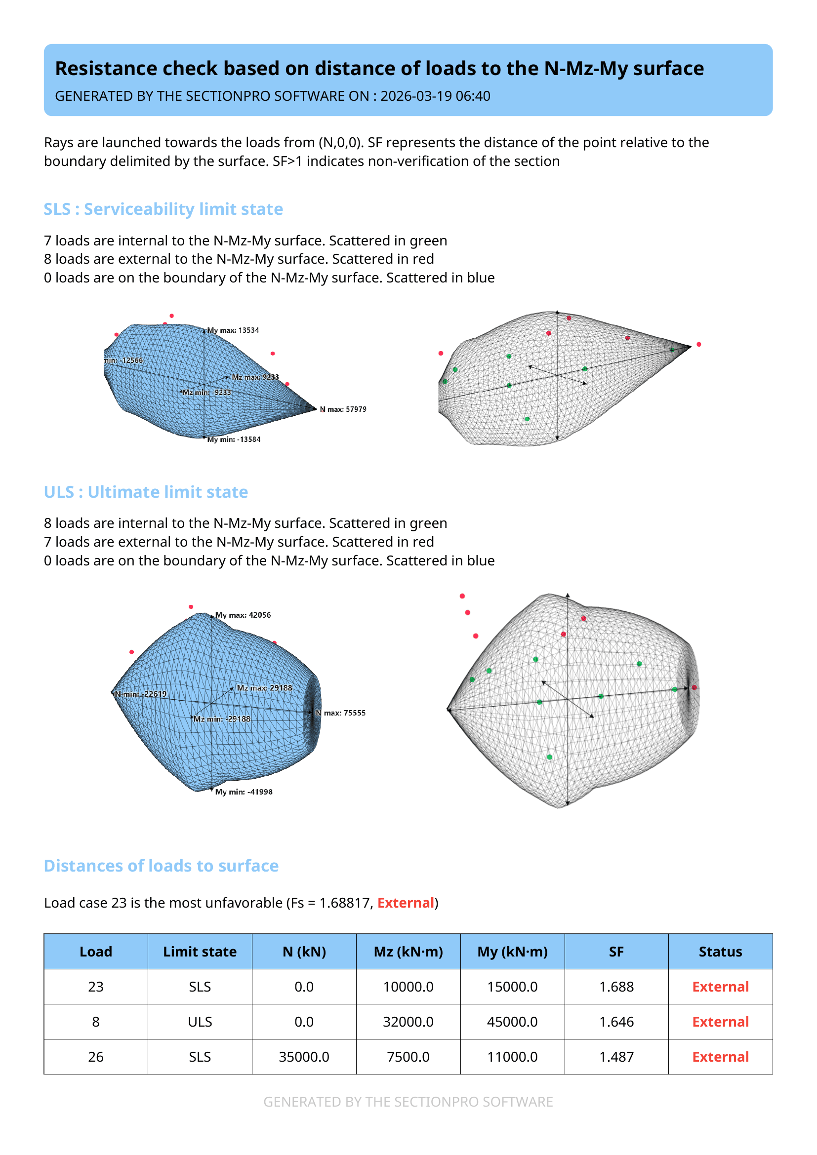
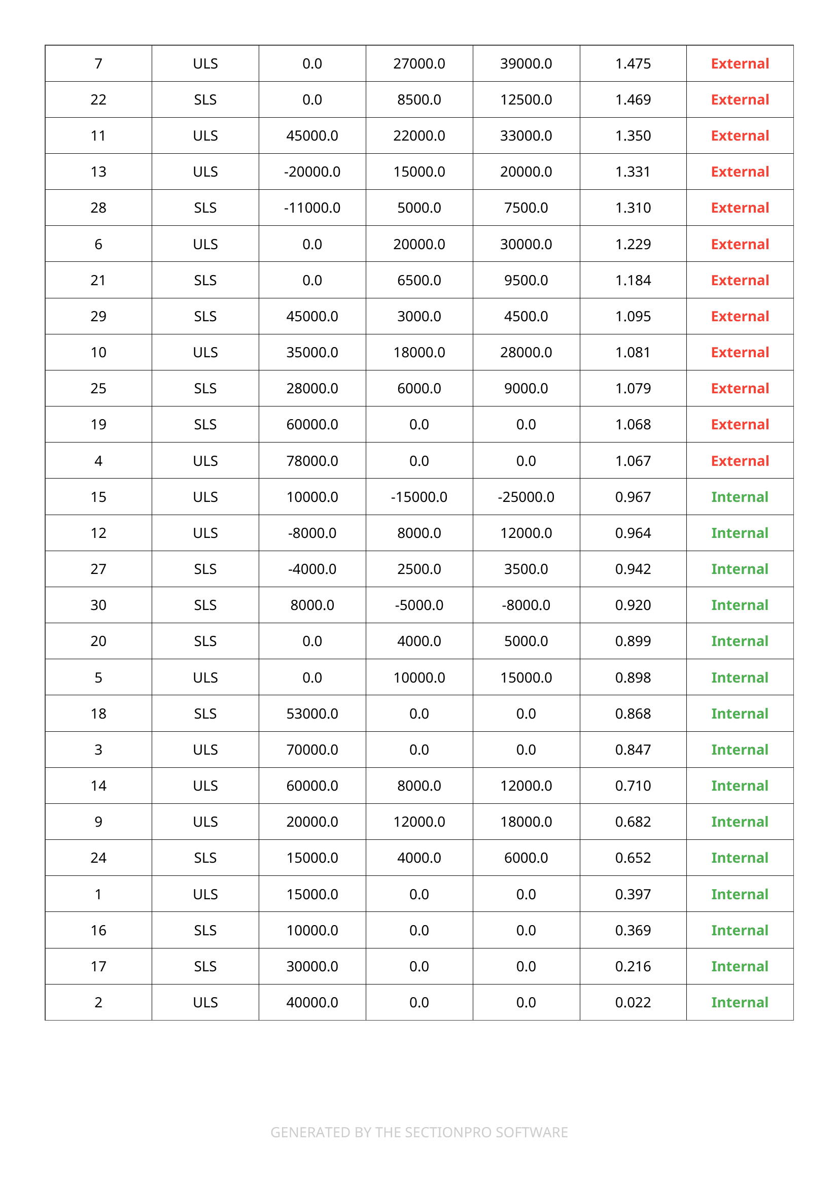
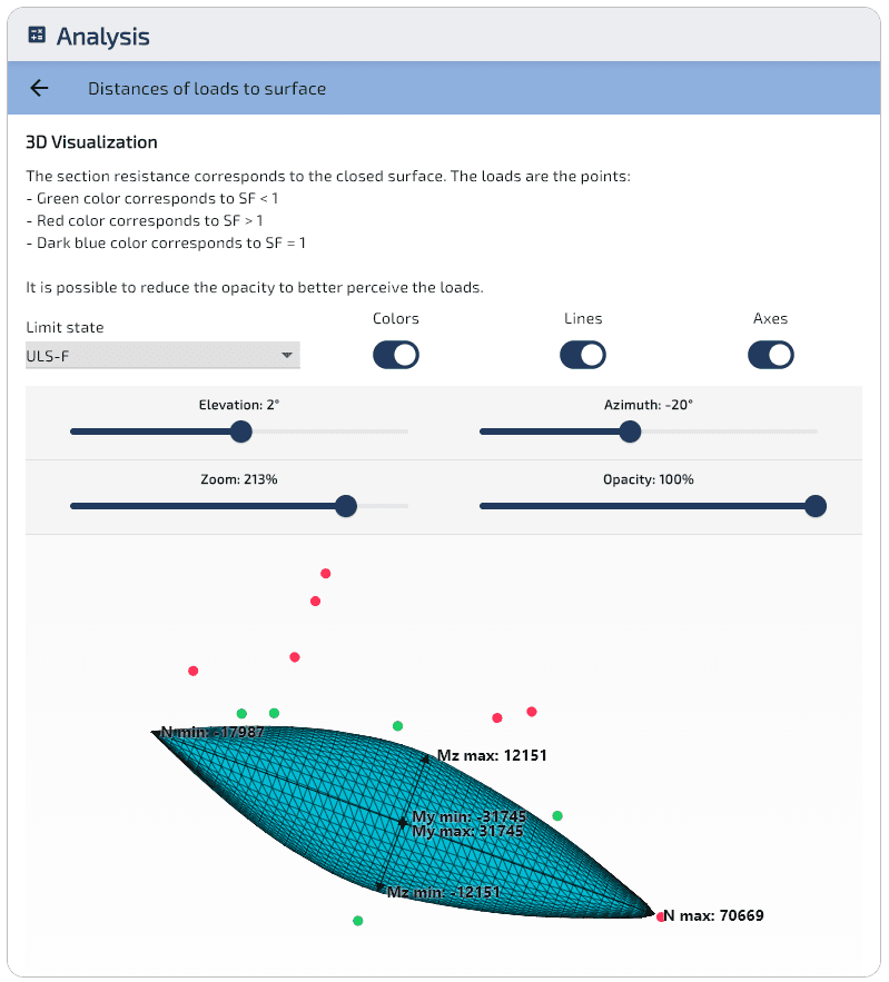
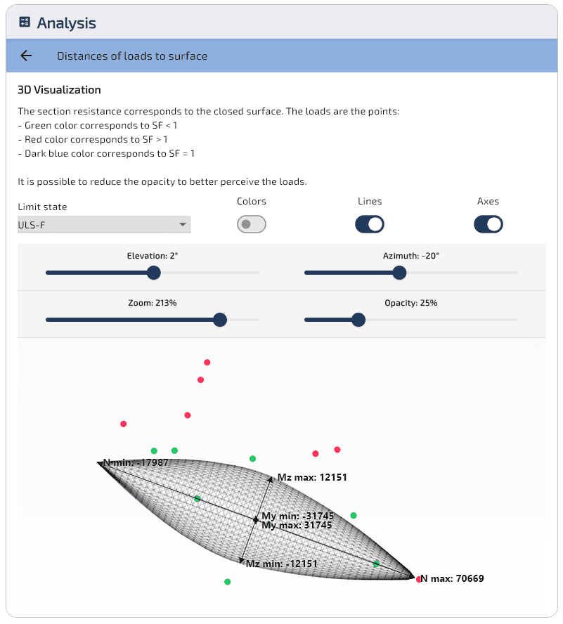
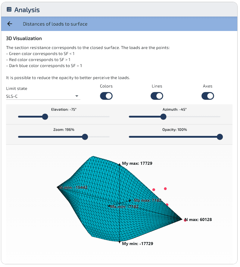
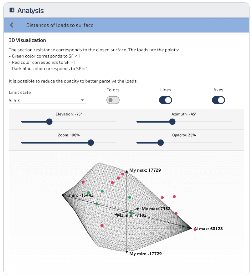
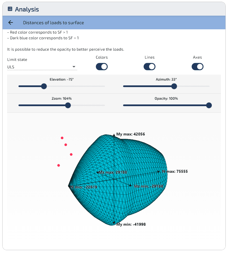
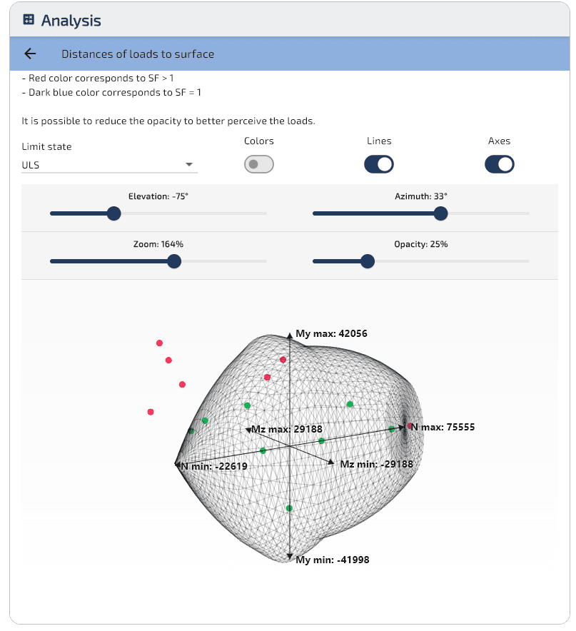
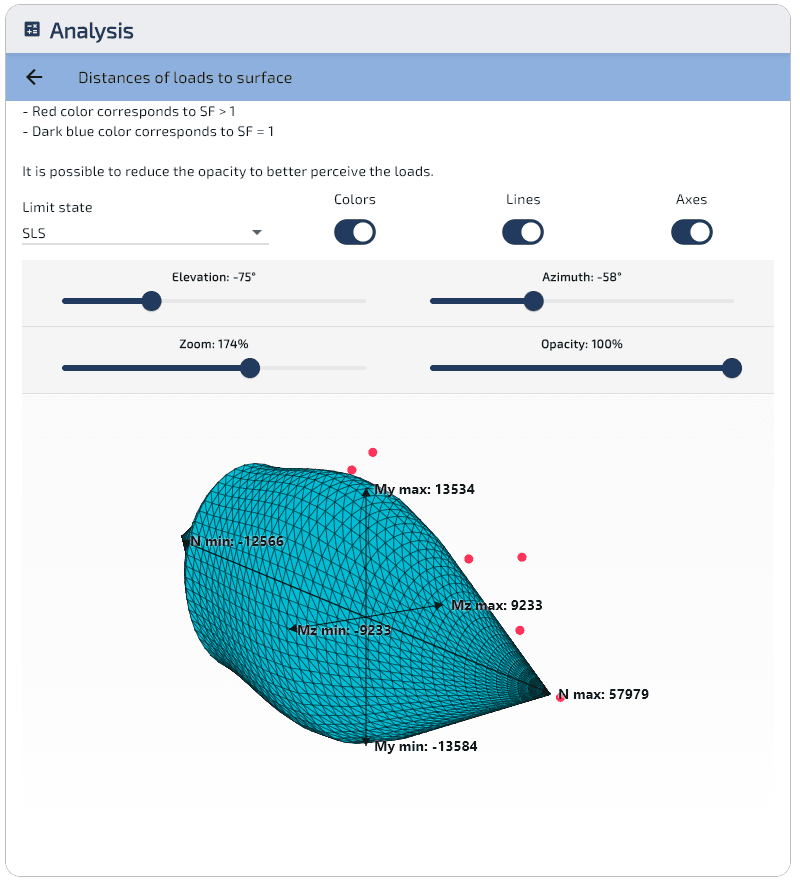
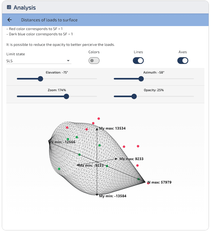
The distances module addresses this by projecting every load point onto the interaction surface and displaying the result as a single 3D scatter plot. For each load, it returns a status (inside, outside, or boundary) and a safety factor quantifying the margin. The engineer sees all combinations at once: one glance reveals which loads are safe, which exceed the capacity, and by how much.
An additional advantage concerns codes with equivalent rectangular stress blocks (ACI 318 Whitney block, CSA A23.3, AASHTO). The stress-strain solver must use the alternative realistic law (parabola-rectangle), since a stress block cannot drive an iterative strain solver. The interaction surface, however, is built directly from the Whitney block, making the distances approach more faithful to these codes' primary design law.
The trade-off: unlike the stress-strain solver, the distances module does not return the deformation state or stress distribution. It answers "pass or fail, and by how much?" but not "what is the stress at each fiber?".
Computed results
SectionPro reports three categories of results for each distance analysis:
Status & safety factor
3D visualization
Exports
This approach vs. the stress-strain analysis
The following table summarizes the key differences between the two verification methods available in SectionPro.
| Criterion | Distances (this article) | Stress-strain (Article \#2) |
|---|---|---|
| Goal | Pass/fail screening | Detailed state |
| Output | + status | , , FS, forces |
| Deformation state | No | Yes |
| Visual output | 3D scatter | Stress/strain diagrams |
| Best for | Large load envelopes | Critical load cases |
| Whitney block | Recommended | Use the realistic law |
| Few loads | Surface overhead | Fast (direct solve) |
| Many loads | Fast (one surface, cheap rays) | Slow (iterative per load) |
Both approaches are complementary. A typical workflow is: (1) use distances to screen an entire load envelope and identify the critical combinations, then (2) use the stress-strain solver on those critical cases to obtain the full section response.
How distances work
Given a load point and the interaction surface , the module computes the centroid of the surface mesh (guaranteed to lie inside the domain) and traces a ray from through until it intersects at a point . The safety factor is defined as:
- : the load point is inside the surface — the section has reserve capacity.
- : the load point is on the boundary — the section is at its exact limit.
- : the load point is outside the surface — the capacity is exceeded.
On the 3D scatter plot, load points are color-coded accordingly: green for internal loads () and red for external loads ().
The surface is computed once per limit state, and then each load point only requires a ray-surface intersection with negligible cost compared to the iterative convergence required by the stress-strain solver.
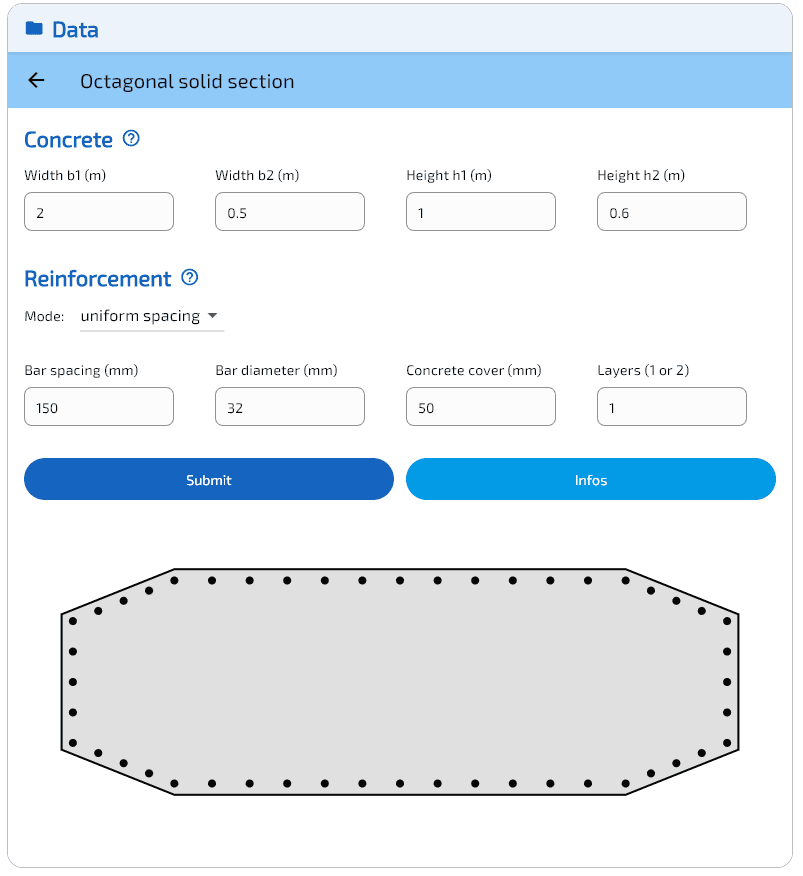
Octagonal section (Eurocode 2)
Input data
The section geometry, reinforcement, and material laws are identical to those used in Article \#4 (Interaction Surface). 30 load combinations are defined: 15 at ULS-F (Fundamental) and 15 at SLS-C (Characteristic), covering a mix of pure axial force, pure biaxial bending, combined loading, tension, and compression.
- Concrete — Octagonal cross section, m, m, m, m.
- Reinforcement — 48 bars, uniform spacing 150 mm, diameter mm, cover 50 mm.
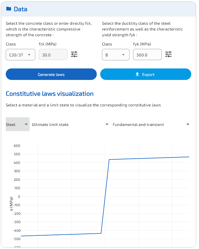
- Material laws (EC2) — Concrete C30/37: MPa, Steel B500B: MPa.
ULS-F (Fundamental)
15 load combinations: 8 internal, 7 external.
| Load | (kN) | (kN·m) | (kN·m) | (−) | Status |
|---|---|---|---|---|---|
| 8 | External | ||||
| 7 | External | ||||
| 4 | External | ||||
| 5 | Internal | ||||
| 3 | Internal | ||||
| 2 | Internal |
Load \#4 ( kN, pure compression) barely exceeds the surface with , confirming that the bounding box kN reported in Article \#4 is correct. Load \#2 ( kN, pure compression) is deep inside the domain (), as expected for a load well below .
The combined loads show the non-cubic shape of the interaction surface: load \#8 (, ) has individual moment components below the bounding box limits (, ) but their combination pushes the point outside the surface ().
SLS-C (Characteristic)
15 load combinations: 6 internal, 9 external.
| Load | (kN) | (kN·m) | (kN·m) | (−) | Status |
|---|---|---|---|---|---|
| 23 | External | ||||
| 26 | External | ||||
| 19 | External | ||||
| 27 | Internal | ||||
| 18 | Internal | ||||
| 17 | Internal |
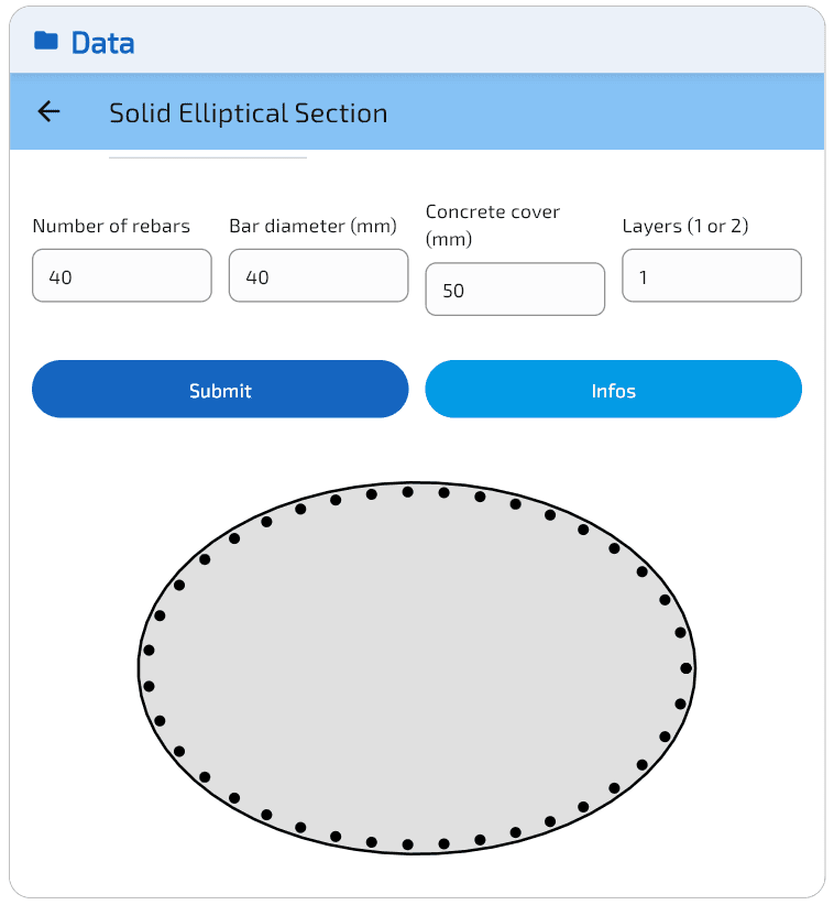
Elliptical section (ACI 318)
Input data
The section geometry, reinforcement, and material laws are identical to those used in Article \#4. 30 load combinations are defined: 15 at ULS and 15 at SLS.
- Concrete — Elliptical cross section, width m, height m.
- Reinforcement — 40 bars along the perimeter, diameter mm, cover 50 mm.
- Material laws (ACI 318) — Concrete: MPa, Steel: MPa.
ULS
15 load combinations: 8 internal, 7 external.
| Load | (kN) | (kN·m) | (kN·m) | (−) | Status |
|---|---|---|---|---|---|
| 8 | External | ||||
| 7 | External | ||||
| 4 | External | ||||
| 15 | Internal | ||||
| 3 | Internal | ||||
| 2 | Internal |
The ACI -factors ( to ) and the cap reduce the nominal capacity, making the ULS surface smaller than a raw interaction surface. From Article \#4, the bounding box gives kN, kN·m, kN·m: exceeding any of these limits guarantees failure, as seen for loads \#4 and \#8. Load \#7 (, kN·m), however, stays within all three limits yet still falls outside the surface () — the bounding box cannot catch this case, the 3D surface can.
SLS
15 load combinations: 7 internal, 8 external.
| Load | (kN) | (kN·m) | (kN·m) | (−) | Status |
|---|---|---|---|---|---|
| 23 | External | ||||
| 26 | External | ||||
| 19 | External | ||||
| 27 | Internal | ||||
| 18 | Internal | ||||
| 17 | Internal |
At SLS, the concrete is limited to the allowable stress ( MPa), resulting in a much smaller surface than ULS. Load \#23 is the most unfavorable across both limit states (): the combined biaxial bending (, kN·m) far exceeds the SLS capacity, even though each moment component individually would be within the bounding box.
Cross-validation with the stress-strain solver
The distances module projects load points onto a pre-built mesh of the interaction surface. The stress-strain solver (Newton-Raphson, Article \#2) iterates to find the equilibrium strain state for each load individually. The two methods should agree: a load inside the surface () must satisfy all material strain limits, while a load outside () must violate at least one limit.
15-load comparison (octagonal section, ULS-F)
For each load, the table gives the distances result ( and Internal/External status), followed by the stress-strain solver output: worst concrete strain and steel strain (both in ‰, absolute values), and the corresponding material verdict.
| Load | (kN) | (kN·m) | (kN·m) | (−) | Status | (‰) | (‰) | Verdict |
|---|---|---|---|---|---|---|---|---|
| 1 | Internal | OK | ||||||
| 2 | Internal | OK | ||||||
| 3 | Internal | OK | ||||||
| 4 | External | KO | ||||||
| 5 | Internal | OK | ||||||
| 6 | External | KO | ||||||
| 7 | External | KO | ||||||
| 8 | External | KO | ||||||
| 9 | Internal | OK | ||||||
| 10 | External | KO | ||||||
| 11 | External | KO | ||||||
| 12 | Internal | OK | ||||||
| 13 | External | KO | ||||||
| 14 | Internal | OK | ||||||
| 15 | Internal | OK |
The two methods are fully consistent. Every External load is confirmed at failure by at least one material (concrete, steel, or both), and every Internal load satisfies all strain limits. The safety factor is a reliable indicator of margin: loads deep inside the surface show strains well below their limits, while loads near the boundary approach them and loads well outside exceed them by a large margin. Loads 10–11: concrete crushing only, steel within rupture limit. Loads 6–8 and 13: both limits exceeded simultaneously.
100,000-load benchmark
To quantify agreement at scale, both methods are applied to 100,000 random load combinations ( kN, kN·m, all at ULS-F). The surface is built once (31 ms) and reused for all distance queries.
| Method | Loads | Query time | Rate | Internal | External |
|---|---|---|---|---|---|
| Distances (queries only) | ms | M/s | % | % | |
| Stress-strain NR | ms | M/s | % | % |
Agreement: 99.97% (99,974 out of 100,000 loads classified identically). The 26 disagreements all have : these load points lie within 0.2% of the surface boundary and are effectively at the limit by any measure.
This is expected behaviour. The distances module does not apply a strict equality test : any load with sufficiently close to 1 is treated as a boundary case. In this narrow region, the two methods can legitimately disagree — the distances result depends on the mesh resolution (finite triangle size introduces a geometric approximation), while the NR solver iterates to exact equilibrium. In such cases the NR solver is the final arbiter: it computes exact equilibrium and its verdict takes precedence over the distances classification.
From an engineering standpoint, whenever , the engineer should not rely on the automatic Internal/External classification alone. The appropriate response is either to run a full NR calculation for a precise verdict, or, better, to modify the section geometry or reinforcement to achieve a clear safety margin ( comfortably below 1).
The distances module is 15 times faster than the NR solver for this batch (query phase). In practice, however, both methods are effectively instantaneous for the vast majority of engineering use cases. The speed advantage becomes meaningful for advanced applications (structural optimisation loops, parametric studies, automated code-checking over large load envelopes) where millions of combinations or more must be evaluated repeatedly.
Conclusion
The distances module provides a fast and reliable method to screen any number of load combinations against the interaction surface of a reinforced concrete section. For each load, it returns a normalised safety factor and an Internal/External status, giving the engineer an immediate picture of the most critical combinations across all limit states simultaneously.
The cross-validation on 100,000 loads confirms 99.97% agreement with the Newton-Raphson stress-strain solver. The 26 disagreements are all located within 0.2% of the surface boundary, where mesh discretisation makes the classification uncertain; in these cases the NR solver remains the final arbiter. For loads clearly inside or outside the surface, the two methods are fully consistent.
Both methods are instantaneous for routine engineering work. The distances approach becomes especially valuable when millions of combinations must be evaluated (optimisation loops, parametric studies, automated code-checking), where its surface-reuse architecture eliminates redundant computation entirely.
Beyond the numerical results, the key advantage of the distances module is the 3D scatter plot: for each limit state, all load combinations and the full resistance domain are visible in a single figure. At a glance, the engineer sees which loads are safe, which exceed capacity, and by how much — a self-contained graphic that integrates directly into a calculation report.
Export
SectionPro exports the distance results in three formats. The PDF report includes 3D views of the interaction surface with scattered load points. For each limit state, the most critical load is identified, followed by a results table sorted by descending . The Excel and text exports provide the same tabular data for external post-processing.