

Introduction
The fire verification of a reinforced concrete section relies first on knowing the temperature at every point of the section after a given exposure duration, for example 30, 60, 90 or 120 minutes. This spatial distribution, the thermal field, governs the rest of the calculation: the strength loss of the concrete and the steel, then the residual load-bearing capacity, follow directly from it. It nevertheless constitutes a self-contained thermal step, which SectionPro solves and reports independently of the mechanical verification.
This article is limited to this thermal step. It recalls its fundamentals, describes the model adopted in SectionPro, then compares the results with the reference profiles of Annex A of EN 1992-1-2.
The thermal problem
Transient heat transfer in the section obeys the nonlinear heat equation:
The thermal properties of concrete vary with temperature. The conductivity decreases monotonically, while the specific heat shows a marked peak around 115 °C, associated with the vaporization of free water and of an amplitude that is greater the higher the moisture content. This peak absorbs a significant part of the flux and markedly delays the progression of the heat front towards the core of the section.
On the exposed faces, the net flux combines convection and radiation:
where is the gas temperature (fire curve), the surface temperature, W/m²K and (default values, adjustable). The unexposed faces are assumed adiabatic ().
The standardized ISO 834 fire curve gives the gas temperature:
These equations involve several parameters: the fire curve, the material's and laws, the surface exchange coefficients. They take by default the values of EN 1992-1-2 and remain editable as input.
The thermal field in SectionPro
SectionPro solves the thermal field on a section of arbitrary shape, whether solid, hollow or made of several materials, without being restricted to the geometries tabulated by the code. Its main capabilities:
- Fire curves. ISO 834 (standard fire), hydrocarbon, external curve, or a user-defined curve as time-temperature points.
- Exposure by face. Each face is exposed or not independently. A beam cast into a slab has three faces exposed to fire, the top face remaining adiabatic; a column has four.
- Protections. A protective layer can be defined face by face (thickness , conductivity , density , specific heat ): gypsum boards, sprayed coatings or insulation. Its thermal resistance enters the boundary condition.
- Materials and geometry. Siliceous or calcareous concrete, moisture content, density and conductivity bound are adjustable. The section can include holes and cavities, multi-material zones and embedded steel.
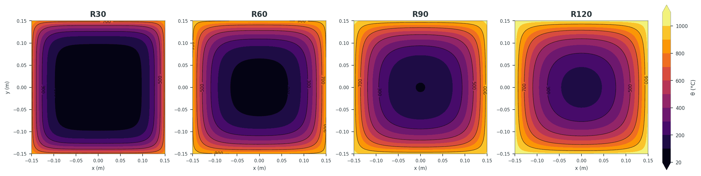
At each requested time step, the full temperature field is obtained: isotherm map, temperatures at the reinforcement and summary quantities (maximum surface temperature, mean temperature, core temperature). These data then serve as input to the residual capacity calculation, which is the subject of the companion article.
Validation against Annex A of EN 1992-1-2
Annex A of EN 1992-1-2 provides reference temperature profiles for common sections exposed to the ISO 834 standard fire: a slab (Fig A.2), beams (Fig A.3 to A.10) and columns (Fig A.11 to A.20). These profiles were established for a moisture content of 1.5% and the lower conductivity bound. These are the assumptions we adopt as the validation reference.
Two geometries representative of the code are reproduced with these same assumptions: the slab, a one-dimensional case exposed on one face, and the column exposed on its four faces, for which the code directly provides the position of the 500 °C isotherm delimiting the concrete considered to remain load-bearing. On each diagram, the isotherms computed by SectionPro, in red, are superimposed on the profiles published in Annex A, in black, plotted in the same frame. The comparison thus bears directly on the same curves.
Heat transfer in the slab remains almost one-dimensional from the exposed face, while the column develops a doubly symmetric field whose cold core shrinks as the exposure continues.
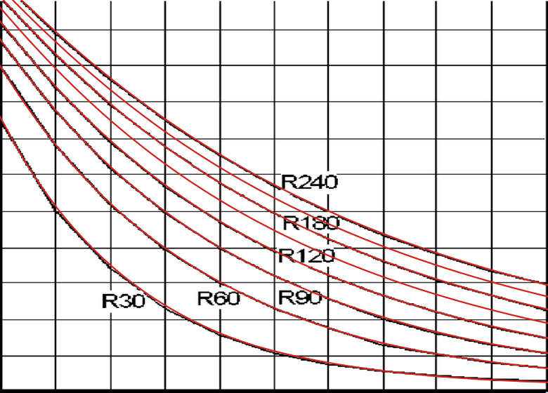
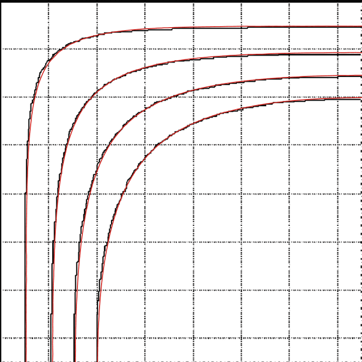
Validation summary. On the slab, the reference one-dimensional case, the computed profile coincides with that of Fig A.2 over the whole range of useful concrete covers as well as down to the core. On the column exposed on its four faces, the position of the 500 °C isotherm follows the code at each duration. The thermal solver is thus validated on these two exposure configurations.
Application example
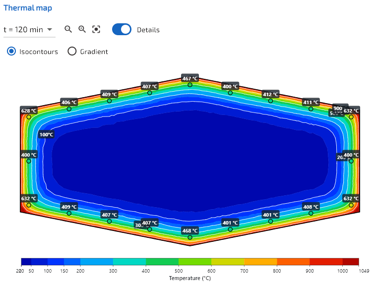
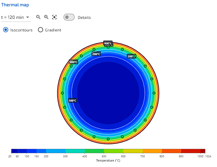
Beyond the shapes tabulated by the code, SectionPro handles arbitrary geometry. The two examples below, a hexagonal section and a circular section, are exposed over their entire perimeter.
Software performance
The thermal field computation is nearly instantaneous: less than a second, including for the longest fire resistance durations. The times measured on the validation cases are reported below.
| Section | Faces | Simulated duration | Computation time |
|---|---|---|---|
| Beam 300 × 160 | 3 | R90 (3 time steps) | 0.12 s |
| Column 300 × 300 | 4 | R120 (4 time steps) | 0.35 s |
| Beam 600 × 300 | 3 | R120 (4 time steps) | 0.52 s |
| Slab 200 | 1 | R240 (8 time steps) | 0.57 s |
Export
The thermal field can be exported as an image (isotherm map, in light or dark theme), in CSV format (node coordinates, nodal temperatures at each time step, reinforcement temperatures) and in the PDF calculation report produced by SectionPro. The output time steps are free, uniform or chosen one by one, which makes it possible to target precisely the regulatory fire resistance durations R30, R60, R90 and R120.
Conclusion
The thermal field is the foundation of any fire verification. SectionPro computes it by transient finite elements, solving the nonlinear heat equation that couples the temperature-dependent conductivity, the specific heat with its moisture peak and the radiation, for an arbitrary geometry and an exposure defined face by face, including protections. The material laws and the fire curve take by default the values of EN 1992-1-2, editable as input.
The comparison with the Annex A profiles confirms this approach: the computed profile coincides with the reference on the one-dimensional case of the slab, and the position of the 500 °C isotherm in the column exposed on its four faces follows the code at each duration. The field thus obtained provides a reliable basis for the calculation of the residual load-bearing capacity in a fire situation.